
As climate change alters the familiar patterns of the planet, it will impact species all across the globe. Among these are Chinook salmon, Oncorhynchus tshawytscha, which are affected by temperature throughout their lives — from eggs to adults. For the Chinook salmon, one looming question is how increasing global temperatures associated with climate change will affect their growth and survival.
I'm Grace Veenstra, a 2023 Hollings scholar, and to answer this question, I built a model framework to simulate salmon life history. Where this model differs from existing ones is in its speed and relative simplicity. These traits ultimately give it the potential to simulate salmon growth and development under different climate and habitat scenarios.
The “King” of salmon
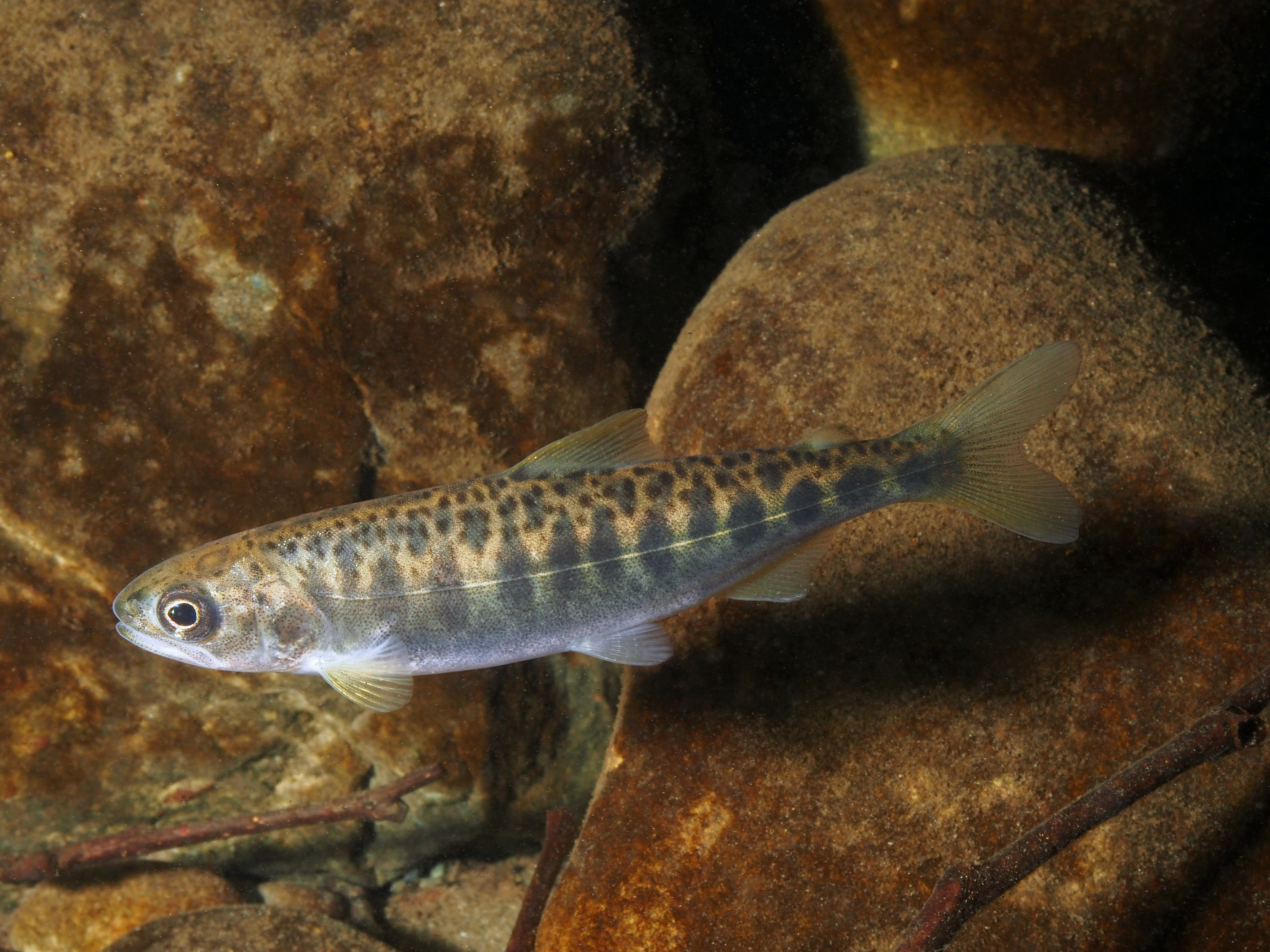
The largest of the seven species of Pacific salmon, Chinook salmon are found along the West Coast of the United States, from California to Alaska. Like many other salmon, Chinook salmon live in freshwater and saltwater, migrating thousands of miles from mountain streams to the ocean and back again.
Nowhere is temperature more important than during the Chinook salmon’s freshwater life stage. In inland streams, the salmon hatch from eggs and spend several years growing to finger-sized juveniles. Temperature affects everything from how fast they grow to how much food they can find.
")
Data on the Salmon River
My model focuses on a threatened group of Chinook salmon that migrate up the Snake River to spawn in central Idaho, in the high mountain streams of the Salmon River watershed.
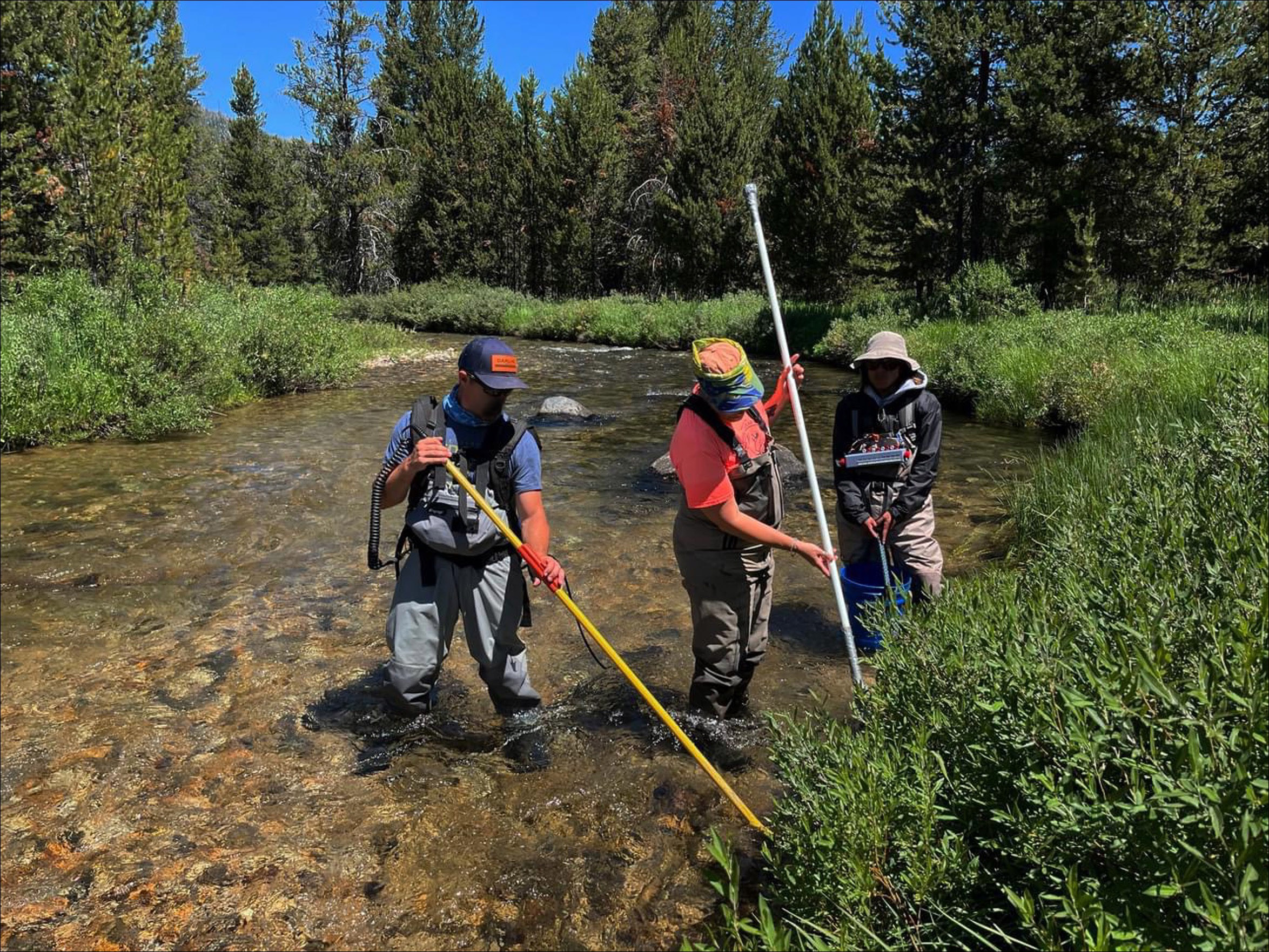
Over several decades, dozens of researchers with NOAA’s Northwest Fisheries Science Center and the Idaho Department of Fish and Game have studied Snake River Chinook salmon. We used the data they collect on salmon size, age, and movement patterns in the model, including:
- Count of redds (nests) made by adults during spawning season to estimate the number of eggs the adults laid.
- Size and tag data from juveniles caught a few months after hatching. The small tracking tags the juveniles are fitted with are used to track their movement patterns.
- Size data from juveniles caught in traps during the downriver migration. Researchers collect, measure, tag, and release fish of all sizes.
- Size and timing data from Lower Granite Dam, which the Chinook salmon encounter on their seaward migration. The dam is 40 miles downriver from the Washington-Idaho border and more than 200 miles from most Chinook salmon spawning streams. Here, researchers record the length, weight, and day of arrival of juveniles.
The models we make using the data allow us to find patterns and predict what we can’t see. For instance, how does the length of salmon vary with temperature? How does survival correlate with size? Through mathematics and computer programs, we can use existing data to make predictions about the future.
")
Making a model
Building the framework
There are many ways to build a model, but no model can do everything. Some of them are very accurate and precise, but require a lot of time and computation power. Others, like the one I used, are well-suited to large-scale scenarios because they are faster and simpler.
I based my model structure on an integral projection model found in a 2018 paper, which simulated beetle phenology. Like salmon, beetles have a complex multi-stage life cycle and temperature-dependent growth. Thus, this previous study was an excellent starting point for a comparable Chinook salmon model.
Filling in the details
Predicting how big salmon could grow isn’t as simple as inputting one rate — I had to use several submodels within the model! These submodels include one for egg development, which determines when the salmon will hatch, and one for the daily growth of juveniles. Each of the submodels’ outputs are based on daily temperature, food intake, and other parameters specific to the Snake River population.
The submodels predict how much the salmon will grow in one day, under one set of temperatures. To stretch this out over years, I use an integral projection model. The integral projection model works by considering both the current size of salmon in the population and how big any salmon could grow, as specified by the submodels. As my model runs, it does this again and again, day after day, ultimately predicting the distribution of future size for the salmon population
Running a model
Different places, different temperatures
There was one more complication to add to my model. As the juvenile salmon get older and bigger, some will move out of their hatching stream into warmer areas downstream, while others stay in their colder stream they hatched in. To account for this, the model has two pathways, a warmer “fall” path and a colder “spring” path, named for when fish move downriver.
Depending on which path a fish follows, they will be located in a different part of the watershed, and thus, the temperature they experience will be different. As mentioned, this impacts how much they grow and the eventual size predicted by the model.
Predicted versus observed
The output of my model is a distribution of the size of juvenile Chinook salmon. To understand these results, we can look at them in a few different ways.
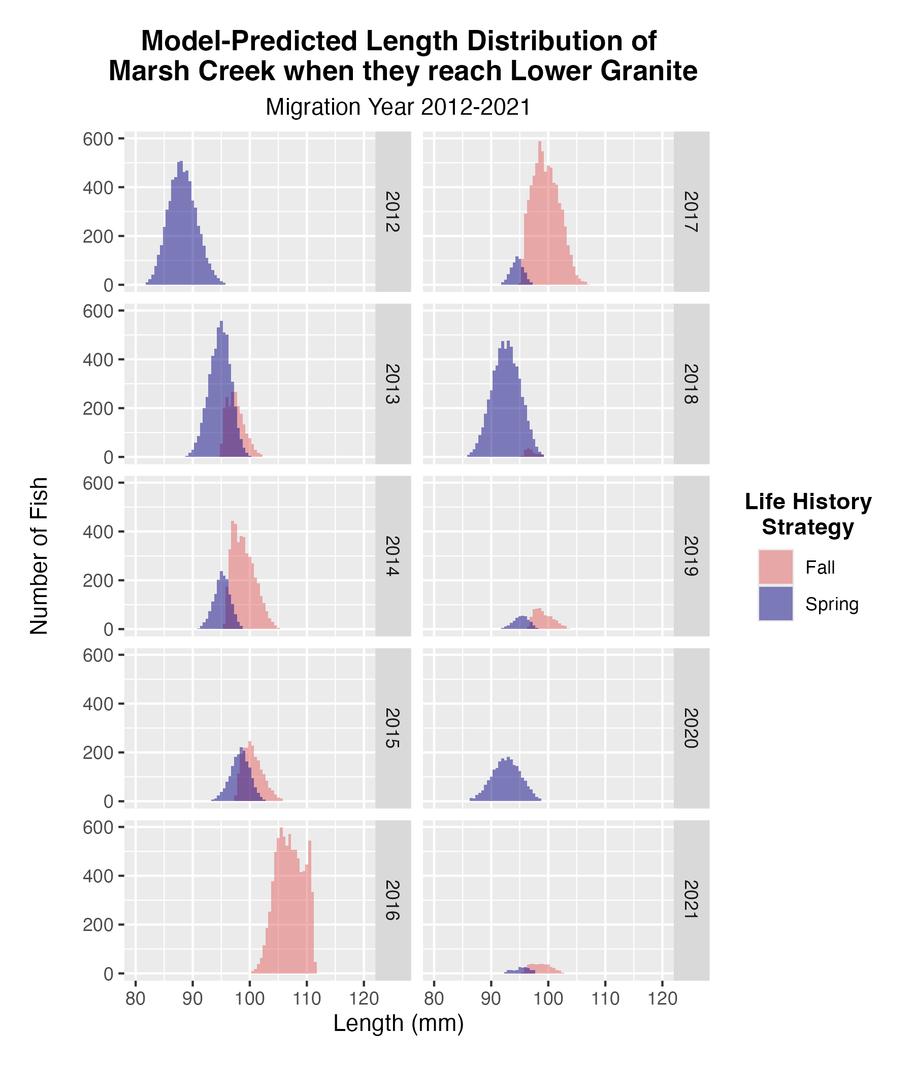
First, I can look at how the model predicts the distribution of size will change from year to year. Will fish be bigger on average in some years than others? Since temperatures are different from year to year, it follows that the resulting distribution of size should also be different. And, we do see this! Depending on the migration year, fish will be predicted to be larger or smaller, and the number that follow the “fall” or “spring” pathway also changes.
.\" Though size distribution varies, they are somewhere between 80 and 115 millimeters. Fall size distributions usually overlap with spring distributions, but are larger. (Image credit: Grace Veenstra)")
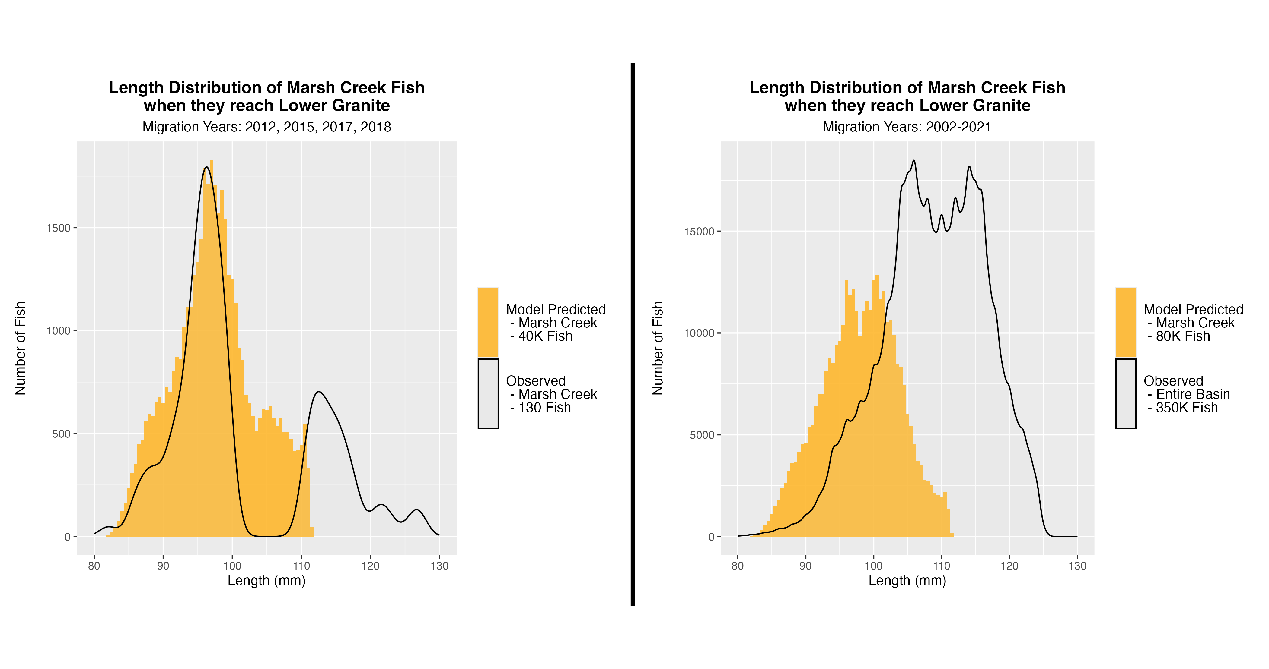
Second, I can compare my model results to real-world observations from researchers, to ensure the model is making accurate predictions. We have data on size and arrival time when fish reach the Lower Granite Dam. I ran the model until the approximate dates juveniles should reach the dam and looked at the predicted body size of juveniles. Specifically, I looked at juveniles from Marsh Creek, a very cold stream, and compared my results to observed data. Then I compared the predicted size distribution of fish from Marsh Creek to fish from the entire Salmon River.
")
Ultimately, my model was a resounding success! Not only was I able to complete a functioning model during my internship, it is getting fairly accurate predictions, despite the limited number of variables it uses.
Where we’re using models
At present, the model is still being tested and is not ready to handle climate scenarios. However, using the model framework and code that I worked on, the integral projection model is already being incorporated elsewhere. With guidance from myself, another intern on this project, Katie Hippe, used my framework to model the juvenile Chinook salmon as they travel through the marine environment.
The value of the integral projection model is its speed and simplicity. For a single spawning year, the model can run in half a minute what might take another model hours. As the climate changes, it is becoming increasingly important to understand the effects it will have on species worldwide. And for the Chinook salmon, this model represents a small step in the right direction.
Grace Veenstra, 2023 Hollings scholar
Grace is 2023 Hollings scholar studying computational biology and science communication at the University of Alaska Fairbanks
")
")